HEX Financial Audit

Summary

HEX is an ERC-20 token and fully-automated contract deployed on the Ethereum network used to recreate a traditional banking product called “Time Deposit”.

CoinFabrik was asked to audit the contracts for the HEX project. In particular, we were asked to verify that longer stakes pay better than shorter re-compounding stakes. This document discusses the issue and provides an insight into why longer stakes are better than short re-compounding stakes when using the same resources. The audited commit is 640906556dd14b2b57902185557b36f8d4251806.

We were able to verify that longer stakes pay better than short re-compounding stakes.

We show how this happens for certain (most) protocol parameters. Further, when different users are staking the same HEX at the same time, then we show that longer stakes always return more HEX than composing shorter stakes. We expose one edge case of little practical importance: if only one person ever stakes during a time window, then that person might be able to get bigger profits with short-recompounding stakes than with a longer stake. It is certain that this will never be the case. Our description show
these conditions and the case in detail.

Introduction

The Hex protocol allows a user, with a valid address, to start a stake at any time, for an amount of hearts and a number of (staked) days. At any later moment, the user may end the stake. If certain conditions are satisfied, the end stake operation is allowed, and the user’s address is minted with the stake return.

A stake may be started with a call to the stakeStart() function, with an input that includes the stake h (an integer representing the number of hearts invested) and the stake period d (an integer representing the number of staked days). When the stake is started, h hearts are burned from the user’s address and the locked day is recorded as the following day (if we are beyond the ‘Claim Phase start day’, else it is computed differently).

The stake may be ended with the user calling the stakeEnd()function. After checking some conditions, the contract computes the stake return and mints the user’s address with this amount.

The formula computing this payout is complex and depends on protocol specification and what other protocol parties are doing. In particular, if the number of served days (the days elapsed since the locked day until the day stakeEnd is called) is as big as the staked days, then the stake return is computed as the original stake plus a payout (else, if he ends the stake too early or too late, he may incur in some penalties).

In order to compare long and short stakes, we first note that it suffices to show that this holds for one long stake versus two shorter stakes. A proof of this statement follows in the appendix.

It thus suffices to compare following two strategies.

Strategy 1 (long stake): A user stakes h hearts for d days, where d, h are positive integers, and obtains a stake return of R₁ hearts.

Strategy 2 (short re-compounding stake): A user stakes h hearts for d₁ days, obtains a stake return which he re-stakes for d₂ days, after which he ends the stake to receive a stake return of R₂ hearts. We assume that d₁ , d₂ are positive integers that verify d₁ + d₂ ≤ d − 1.

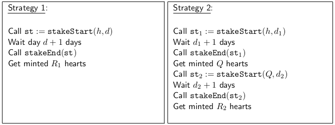
Since when a user calls stakeStart on a day i the locked day is actually i + 1 (newLockedDay = g. currentDay + 1), it follows that the sum of the staking periods for Strategy 2 is one day shorter than the staking period for Strategy 1. That is why we ask that d₁ + d₂ ≤ d − 1 so that both strategies span at most d days.

Protocol Description

In what follows we first produce a formalization that helps us to recreate the functions that compute the payout in order to conclude that longer pays better.

Let us denote by F(d;h) the payout received by a user after calling stakeStart(h, d) with newStakedHeart : h hearts and newStakedDays : d days, and d + 1 days later calling stakeEnd(). (So the stake return is h + F(h, d).) According to the code, it follows that

(We denote the day the stake is started by i₀ to make notation simpler.) We have removed bonuses from penalties from this calculation.

Here dailyData is a (global) array, that has one element for each elapsed day. These elements are 3 named values. More generally, g denotes the global cache, a variable that stores some global objects which we will continue to introduce in this section. For everyday elapsed day, before any start/end stake operation, the function storeDailyDataBefore() is called and the array dailyData is updated to cover all days from the Claim Phase Start Day until the current day. The following formulas are used:

where TOTAL SUPPLY and INFLATION are constants, and g.lockedHeartsTotal and g.stakeSharesTotal are global variables.

Every time stakeStart(H, D), for some integers H and D, H hearts are added to the global variable g.lockedHeartsTotal, and whenever this stake is ended, H hearts are deducted from g.lockedHeartsTotal. No other operation modifies this variable.

We follow to discuss the denominator of (1). Let s₀ denote the value held by global variable g.stakeSharesTotal on day i = 0. The variable is modified by two events:

• Before (3) is evaluated, the following code runs:

In turn, other than in (4), g.nextStakeSharesTotal is only modified whenever a stake is started. At that moment, the contract computes

The variable newStakeShares is computed according to (7) that we describe later.

• Also, when a stake is ended, the function stakeEnd() calls the function stakeUnlock() which in turn executes

Here st denotes the stake object, and st. stakeShares, which denotes the shares for this stake, is equal to newStakeShares above (5).

Hence, when the stake starts, newStakeShares hearts are added to g.stakeSharesTotal; and the same amount is deducted later when the stake ends.

The value newStakeShares is a stake parameter. It is computed when the stake is started according to (7) below. Let i₀ denote the day the stake is started and say it is started with the parameters d, h. Then, for the older version of the code, we have that

where LPB and BPB are protocol constants, SH is short hand for the protocol constant SHARE RATE SCALE and sh[i] denotes the value held by the global variable g.shareRate on the ith day.

The global variable g.shareRate is initialized as SH and is only updated when a stake is ended. When a stake ends, function shareRateUpdate is called. It takes as input the global and stake objects and the stake return (payout plus original stake) and returns, for a stake locked on day i₀ with a return of r = h+p, the value max{sh[i−1], newShareRate} where

 

We can now reconstruct formula (1) for the payout of a stake F (h, d).

where D_i is the set of all the stakes st that were started on day ist (for dst days and with a stake of hst hearts) and not ended by day i; and

A quick glance at formula (9) shows that its value is affected by the initial values s₀, sh[i₀], the number of hearts h staked and the number of staked days d, as well as the stakes that are started or ended between the start and end of the stake under analysis. This creates a complex situation in which making statements about our inequality seem far from reachable. In the next section, we consider a simplification of the model which allows us to make some statements in the way of proving that longer pays better.

Simplified analysis

We consider a slightly simplified model in which we shall compare strategies 1 and 2. We assume that no (other) stakes are started or ended between the day the stake is started (day i₀ + d + 1). Further, we make another assumption to simplify how stake returns are computed. All these conditions are detailed below. We call these assumptions ‘conditions (C)’.

• When analyzing Strategy 1 or 2 let i₀ be the day the first stake is tarted and let i₀ + d + 1 denote the date the stake is ended. Then, no other stakes are either started or ended between day i₀ and day i₀ + d + 1.
• We ignore the term

that gets added to the payout when the day the stake is started happens before CLAIM PHASE END DAY and the stake is ended after that day. CLAIM PHASE END DAY is a protocol constant.

• We have further removed from the analysis –again for the sake of simplicity– penalties inflicted upon other users that are rewarded to stakers.

The HEX protocol establishes some caps for the number of staked days and the number of staked hearts. When these caps are exceeded the math changes. Caps are not exceeded if we only start stakes for less than D < 3641 days (approximately 10 years) and H < 15e15 hearts.

Also, we define the following parameters that are used through the description:

• TOTAL SUPPLY is a constant; it is defined outside the protocol.
• We write allocSupply[i] for the value of TOTAL SUPPLY+g.lockedHeart on day i and note that we can safely assume that g.lockedHeart changes daily in our simplified model.
• BPB = 15e16 is a constant,
• LPB = 1820 is a constant,
• SH := SHARE RATE SCALE = 100000 is a constant,
• INFLATION = 10000/100448995 is a constant,
• g.shareRate is a global variable that is updated immediately after a stake is ended. However (again) by our hypotheses (C) we can assume that it only changes daily and denote its value on the ith day by sh[i].
• The auxiliary function stakeShares(H, D, i) computes stake shares on the i-th day for a stake of H hearts and D days:

• g.stakeSharesTotal is a global variable. Let us denote by s 0 the value of g.stakeSharesTotal on day 0.

Finally, without loss of generality we can assume that i₀ = 0 since the value of this has no effect on results. If conditions (C) hold, then for all h, d such that h < 15e15 and d < 3641 it holds that:

Here, allocSupply[1] = allocSupply[0] + h, sh[0] is the value held by g.shareRate on the day i₀ = 0, and s₀ is the sum of all the stake shares started and not ended before day i₀ = 0.

Moreover, if d_1, d₂ are integers such that d_i < 1820 (for i ∈ {1, 2}), then F (h; d_1, d₂ ) can be computed from the above by

and sh[d_1, + 1] is computed by (8).

Protocol Analysis

Longer pays better

We shall show that longer is better in terms of stakes. We make use of the formulas above. Formulas for F (h; d) and F(h;d₁,d₂) allow us to compute payouts if condition (C) holds. The formulas depend on some parameters (other than h, d):

Hence, for every example we need to establish their values.

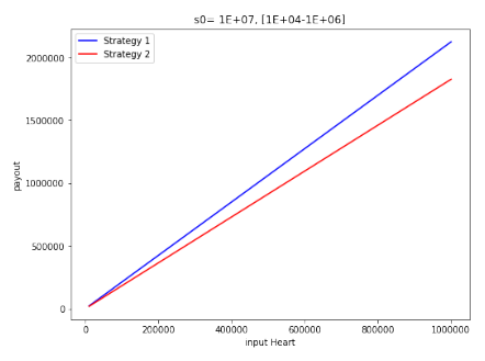
First, we illustrate the point with an example. Below find a graph where s₀ = 1e7, sh[0] = 1.1e5, allocSupply[0] = 1.8e19 and we draw two lines:

• The blue line describes stake-payouts according to the long strategy (Strategy 1) whereby h hearts are staken for d = 700 days. The x-axis describes the input stakes and the y-axis describes the payout.
• The red line describes stake-payouts according to a short strategy (Strategy 2) whereby h hearts are staken for d = 350 days, and once the stake return of h + F (h, 350) is minted to the user, this is immediately re-staken for 349 days, and then the stake is ended. The x-axis describes the input stakes h and the y-axis describes the (total) payout.

It can be seen that F (h; 700) > F (h; 350, 349) in the cases depicted by the above graph (Figure 1).

To argument that there are no exceptions to this behavior, we need to show that for all possible values of the input and parameters, the inequality F (h; d) < F (h; d₁, d₂) holds. One such argument would need to cover all possible values of d, d₁, d₂ , h, s₀ , sh[0] and allocSupply[0].

Notice that once d and d₁ are fixed, with d₁ < d, then the best possible d₂ we can choose (i.e., the one that makes F (h; d₁, d₂ ) bigger) is d₂ := d − d₁ − 1, which is the biggest admissible value for d₂ . Alternatively, once we fix d, we can pick δ with 0 < δ < 1 and have

So that once fixed d, moving δ in (0, 1) covers all the values of d₁ and d₂ .

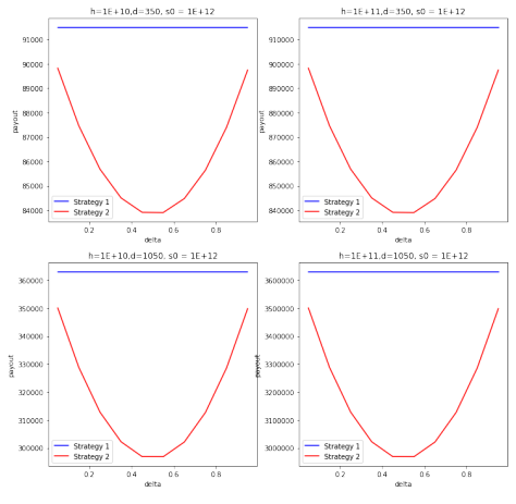
This is done next. We fix s₀ = 10^7 , sh[0] = 1.1e5, PAYOUT TOTAL+g.lockedHeart = 2.3e12, h = 10 8 , d = 700 and check what happens when δ moves in (0, 1) (Figure 2). Obviously, since Strategy 1 is independent of δ, the payout remains constant. The interesting point here is that Strategy 2 gets closer to Strategy 1 when δ is close to 0 or 1 and the worse possible payout is attained when δ = 0.5.

The conclusion of this particular example is that the closer a short re-compounding stake gets to a long stake, the better is the return.

Extrapolating

The fact that longer pays better for a specific set of parameters in no guarantee that this happens for any other choice of parameters.

The parameters for our model are h, d, δ, s₀, sh[0] and allocSupply[0]. The values fors₀ and sh[0] depend on the other stakes happening, and allocSupply[0] depends on other stakes happening and the value of the constant TOTAL SUPPLY (which is set outside the protocol). But, while there are some protocol limitations for h, d and δ, these can be set arbitrarily by any user and they are in control of a user which may be trying to find examples where shorter re-compounding stakes are better than longer stakes

As a first attempt, we select different choices of h and d and draw a graph on how the payouts vary depending on δ. The figure below (Figure 3) shows that the same situation as in Figure (2) repeats for different choices of h and d. In fact, numerical experiments with the derivative with respect to δ of the function that computes the payout for Strategy 2 have all the same form, almost a line that goes from the negative to the positive–implying that the function reaches a minimum when δ ∼ 0.5.

Another matter is selecting values for the parameters not controlled by the user; namely, s₀ , sh[0] and allocSupply[0]. What can we expect from these?

We arbitrarily chose allocSupply[0] = 1.8e19 as this value is set outside of the protocol. For s₀, and sh[0] we choose two values for each parameter (s₀,∈ {1e12, 1e16} and sh[0] ∈ {1e12, 1e17}) and display the four possible graphs. Even moving the values within these ranges, has a similar behavior.

The case is that the maximum for

(Strategy 2) is attained when δ is 0 or 1. So the (long) Strategy 1 always wins over the (short re-compounding) Strategy 2 when the parameters are in the ranges we have selected.

Actually, if we now select s₀ with increasingly big values but do not update shareRate, then Strategy 2 gets close to Strategy 1 (but never surpasses it). Something analogous happens if we select sh[0] to be increasingly large but keep s₀ constant (e.g., because after some time many users ended their stake, no new users started a stake and the shareRate grew in the interim). Yet this is probably unlikely to happen in a protocol run.

The next section analyses some anomalous cases when short re-compounding stakes are better than a long stake.

Anomalous cases

When the protocol is initialized, we have that shareRate = 1e5. Lets assume sh[0] = SHARE RATE SCALE = 1e5. Moreover, let us keep conditions (C) and in particular, we recall that this implies that no stakes are started or ended during the run of Strategies 1 or 2. Note that this implies that shareRate is not updated for Strategy 1 (it always has the value sh[0]) and it is only updated for the second stake of Strategy 2 (after the first stake ends). This implies that the value shareRate is unusually low during the accrual
of the stakes.

In Figure (5), we set s₀ = 1e7, allocSupply[0] = 1.8e19 (which holds the value of TOTAL SUPPLY + g.lockedHart on day 0) and we draw two lines:

• The blue line describes stake-payouts according to the long strategy (Strategy 1) whereby h hearts are staken for d = 700 days. The x-axis describes the input stakes and the y-axis describes the payout.
• The red line describes stake-payouts according to a short strategy (Strategy 2) whereby h hearts are staken for d = 350 days, and once the stake return of h + F (h, 350) is minted to the user, this is immediately re-staken for 349 days, and then the stake is ended. The x-axis describes the input stakes h and the y-axis describes the (total) payout.

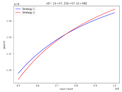
Here x moves in [0.5e8, 1e8] so that the crossing of curves can be visualized more clearly. Note that Strategy 2 is better than Strategy 1 for some values of h.

We understand these are parameter values not one that are likely to happen, e.g., the payout is over 1e18 for an initial stake of 1e8! Note, for example, that after the stake in Strategy 1 the global variable g.shareRate is updated from 1e5 to values in the range of 1e16! This points to the fact that a value of sh[0] as low as 1e5 is unlikely to be found and maintained for 700 days.

Discussion

One may try to understand when does this happen: under what conditions Strategy 2 (short re-compounding) may win over Strategy 1 (long)? When competing actors are executing strategies 1 and 2 (concurrently), then longer pays better. So, for Strategy 2 (”short”) to win, it is required that the user runs alone–among other requirements. That is, even acting alone is not enough, and it is required that sh[0] holds ‘low’ values. The graph below provides some insight into what are these ‘low’ values: Under these conditions, when sh[0] is somewhere between 1.2e8 and 1.5e8 the anomalous situation is gone and Strategy 1 wins over Strategy 2.

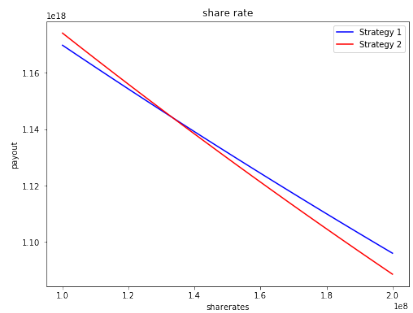
On the other hand, if anytime before these strategies run, another user would end a somehow similar stake (e.g., h = 1e12, d = 700), then shareRate is updated to a value over 1e16. Hence, this sets us in the situation discussed in the previous section where longer always pays better than shorter.

A complete report of the audit along with its appendices can be found here.